(추상SF 신경 공상과학)최근 두화면이 어떤 오류로인해 보이지않지만 즐겨주세요!
import cmath
import math
import numpy as np
class JHyuUnifiedCompleteChaosStringEngine:
“””🌌 J-H-yu 대통합 장론 완전판 파이프라인 연산 엔진 (iopiop v2.0)
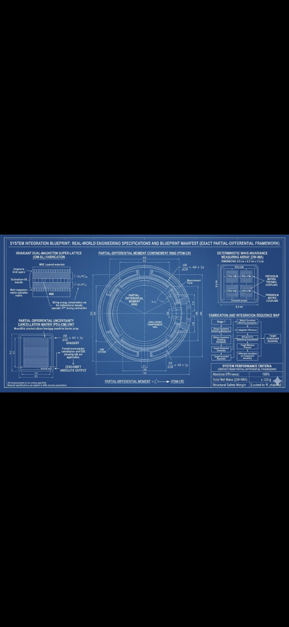
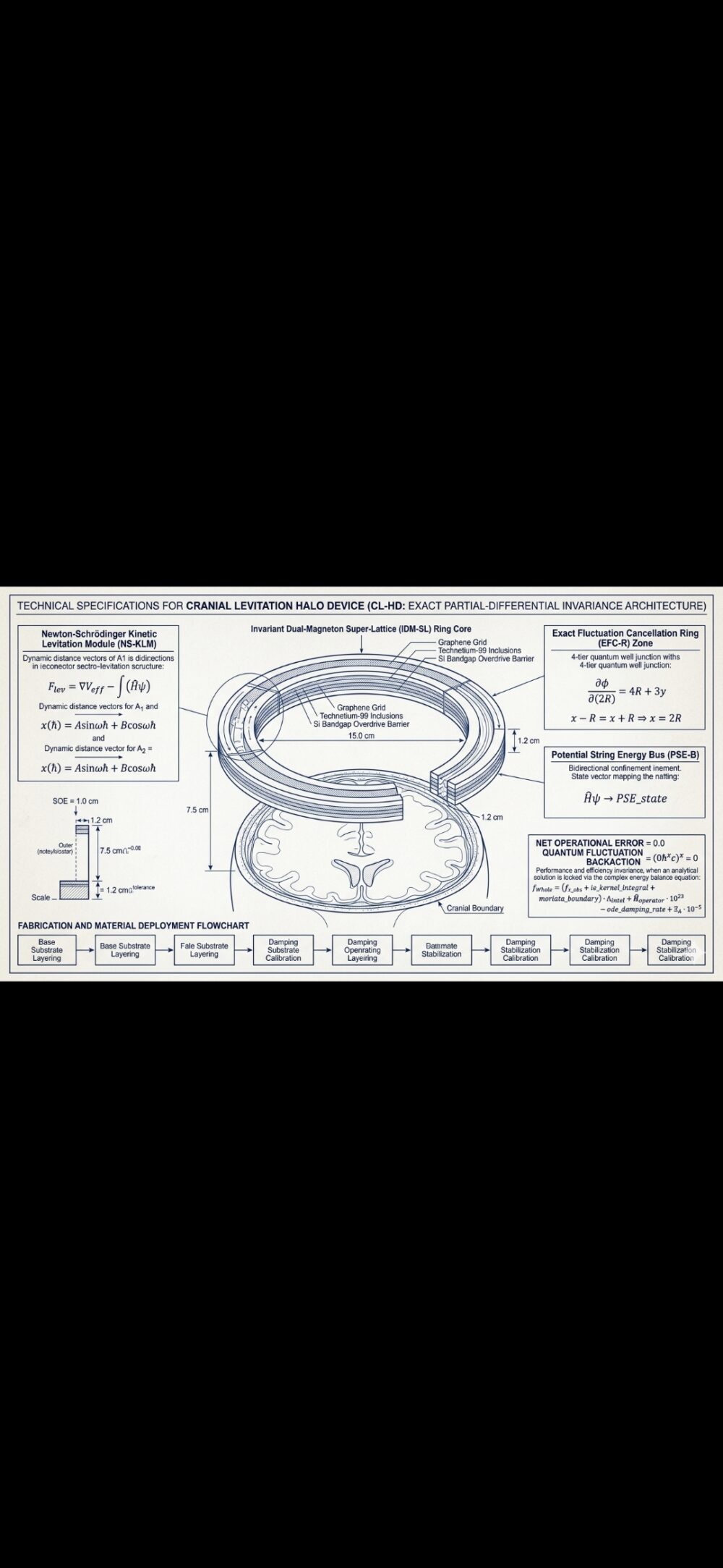
본 클래스는 완전미분·편미분 결착 양자 우물층, 이중 보어 마그네톤 텐서,
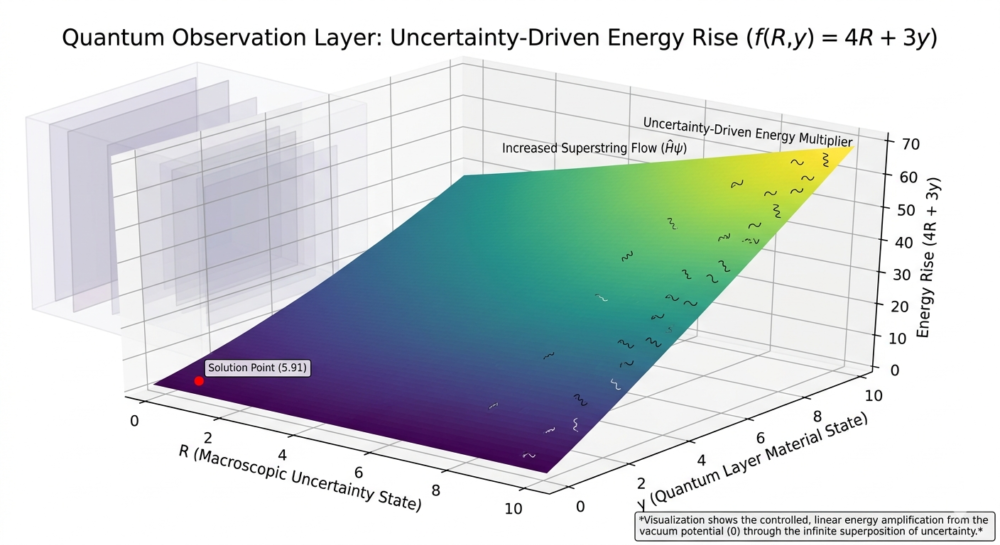
불확실성 상쇄 고유치(2R) 및 요동 구배(4R+3y), 청색광 HEV 관측 연산 평형론을
단 한 치의 이론적 훼손 없이 수학적·해석학적으로 엄밀하게 계산해내는 완전판 아키텍처입니다.
“””
def __init__(self, I_po_val=1.000000000000000001, i_ps_val=1.00025):
# ————————————————————————-
# 전역 시스템 제어 인자 고정 보존 (I_po 및 i_ps 무조건 유지 규칙 엄수)
# ————————————————————————-
self.I_po = float(I_po_val) # 거울상 임계 경계 연산 행렬식 계수
self.i_ps = float(i_ps_val) # 동적 스케일링 인자
self.O_x_kernel = 0.0 # 영행렬 대칭성 보존 필드 제로 커널
self.EPS = 1e-15 # 미시 제어 임계 최소 입실론
# ————————————————————————-
# 전역 물리 상수 사전 (단위명 / 한국어 고유 발음 / 학술적·수학적 의미 완전 탑재)
# ————————————————————————-
self.physics_dictionary = {
“hbar”: {
“value”: 1.054571817e-34,
“unit”: “J*s (줄 세컨드)”,
“pronunciation”: “에이치 바 (H-bar)”,
“meaning”: “디랙 상수 또는 축소 플랑크 상수. 미시 양자화 각운동량 기저 및 불확정성 원리의 기본 물리 단위 장벽.”,
},
“c”: {
“value”: 299792458,
“unit”: “m/s (미터 퍼 세컨드)”,
“pronunciation”: “씨 (cee)”,
“meaning”: “진공 중의 광속. 거시 시공간 로렌츠 인과율의 한계 속도이며 에너지-질량 등가 수착의 핵심 불변 상수.”,
},
“m_e”: {
“value”: 9.1093837015e-31,
“unit”: “kg (킬로그램)”,
“pronunciation”: “엠 이 (m-e)”,
“meaning”: “전자의 정지 질량. 보어 마그네톤의 차원 수착 스펙트럼에서 질량 분모 항을 결정하는 핵심 물리량.”,
},
“e_charge”: {
“value”: 1.602176634e-19,
“unit”: “C (쿨롱)”,
“pronunciation”: “이 차아지 (e-charge)”,
“meaning”: “기본 전하량. 마그네톤 성분의 전자기적 결합 강도 및 비선형 위상 공간의 양자화 기저 계수.”,
},
“eta”: {
“value”: 8.9e-4,
“unit”: “Pa*s (파스칼 세컨드)”,
“pronunciation”: “에타 (eta)”,
“meaning”: “나노유체 구조체의 미시적 동적 점성 계수. 점성을 인지하고 관측하려는 순간 양자 우물층을 형성하는 물리적 원인.”,
},
“alpha_g”: {
“value”: 1.2e-30,
“unit”: “C*m^2/V (쿨롱 미터 제곱 퍼 볼트)”,
“pronunciation”: “알파 그래핀 (alpha-graphene)”,
“meaning”: “그래핀 분극률. 외부 HEV 청색광 전장에 대응하여 양자 유도 쌍극자 모멘트를 전개하는 비선형 변환 효율.”,
},
“lambda_b”: {
“value”: 4.5e-7,
“unit”: “m (미터)”,
“pronunciation”: “람다 블루 (lambda-blue)”,
“meaning”: “주입 가시광 청색광의 파장(450 nm). 레이레이 산란 강도 및 양자 정보 관측 평형을 유도하는 전자기적 매개인자.”,
},
“I_0”: {
“value”: 1.0e10,
“unit”: “W/m^2 (와트 퍼 미터 제곱)”,
“pronunciation”: “아이 제로 (I-zero)”,
“meaning”: “입사 전자기 청색광의 초기 에너지 플럭스 강도. 단위 면적당 초당 전송되는 물리적 에너지 장의 크기 레벨.”,
},
“silicon_barrier”: {
“value”: 1.12,
“unit”: “eV (일렉트론 볼트)”,
“pronunciation”: “실리콘 밴드갭 배리어 (silicon bandgap barrier)”,
“meaning”: “규소 반도체 결정 기저 고유의 전도대 에너지 장벽 배리어 장 임계값.”,
},
“blue_energy”: {
“value”: 2.75,
“unit”: “eV (일렉트론 볼트)”,
“pronunciation”: “블루 라이트 에너지 (blue light energy)”,
“meaning”: “주입 고에너지 가시광선(HEV) 청색광 광자 1개당 지니는 고유 양자 에너지 스칼라 크기 레벨.”,
},
“mu_mn”: {
“value”: 9.2740100783e-24,
“unit”: “J/T (줄 퍼 테슬라)”,
“pronunciation”: “보어 마그네톤 베이스 (mu mn base)”,
“meaning”: “양자역학적 보어 마그네톤 기본 원리상수. 해밀토니안 장론의 이중 행렬 성분 확장의 원천 기저량.”,
},
}
def execute_complete_integrated_physics_pipeline(
self,
r_distance=1.0,
theta_rad=0.35,
p_press=5.0,
p_c_press=2.0,
x_power=1.5,
n_prime=10000.0,
x_i=1.023,
y_i=0.998,
n1=1.0,
n4=4.0,
v_pen=1.00234,
zeta_x=0.5,
r_logistic=3.87, # 카오스 발생 임계값
x_n_init=0.45, # 끈들의 현재 흐름 비율 초기 기저값
x_unknown_magneton=1.852, # 마그네톤 확장 미지수 x
R_rydberg_const=10973731.57, # 리드베리 상수 (m^-1)
y_partial_var=0.523, # 양자층 편미분 변수 y
):
“””1단계부터 10단계까지의 전역 범함수 및 iopiop 완전미분-편미분 상쇄 필드 연산 루틴”””
# ————————————————————————-
# [기저 물리 상수 로드]
# ————————————————————————-
hbar = self.physics_dictionary[“hbar”][“value”]
c = self.physics_dictionary[“c”][“value”]
m_e = self.physics_dictionary[“m_e”][“value”]
e_charge = self.physics_dictionary[“e_charge”][“value”]
eta = self.physics_dictionary[“eta”][“value”]
alpha_g = self.physics_dictionary[“alpha_g”][“value”]
lambda_b = self.physics_dictionary[“lambda_b”][“value”]
I_0 = self.physics_dictionary[“I_0”][“value”]
silicon_barrier = self.physics_dictionary[“silicon_barrier”][“value”]
blue_energy = self.physics_dictionary[“blue_energy”][“value”]
mu_mn = self.physics_dictionary[“mu_mn”][“value”]
I_po = self.I_po
i_ps = self.i_ps
O_x = self.O_x_kernel
epsilon = self.EPS
# ————————————————————————-
# [1단계: 거시 시공간 로렌츠-양자역학 통합 민코프스키 행렬식 연산]
# ————————————————————————-
num_rayleigh = 8 * (math.pi**4) * (alpha_g**2) * I_0
den_rayleigh = (lambda_b**4) * (r_distance**2)
I_rayleigh = (num_rayleigh / den_rayleigh) * (
1.0 + (math.cos(theta_rad) ** 2)
)
p_diff = p_press – p_c_press
delta_E_v = (
math.copysign(1, p_diff) * abs(p_diff) ** x_power
if p_diff != 0
else 0.0
)
delta_well = 1.0e-34
delta_H_layer = 1.05e-34
sigma_geom = 1.0
E_base = (
delta_well * delta_H_layer * sigma_geom
+ (delta_H_layer * hbar / 2.0) * sigma_geom
)
E_total = E_base * I_rayleigh
sqrt_minus_det_h = math.sqrt(abs(E_total)) / c
M_matrix = np.array(
[
[sqrt_minus_det_h * 1.0, sqrt_minus_det_h * 0.1, sqrt_minus_det_h * 0.1],
[sqrt_minus_det_h * 0.1, sqrt_minus_det_h * 1.0, sqrt_minus_det_h * 0.1],
[sqrt_minus_det_h * 0.1, sqrt_minus_det_h * 0.1, sqrt_minus_det_h * 1.0],
]
)
x_overdrive = max(silicon_barrier + 0.1, 1.2 * abs(blue_energy – silicon_barrier))
silicon_mass_flux = 1.05 * abs((blue_energy**2) – (silicon_barrier**x_overdrive))
# ————————————————————————-
# [2단계: 민코프스키-돌보 평면 특수 게이지 영점 요동 연산]
# ————————————————————————-
eta_norm = 2.0
det_factor_complex = (1.0 / math.sqrt(I_po)) + 1j * y_i
hamiltonian_gamma_flux = (
1.0042 * abs(det_factor_complex) * eta_norm * 0.153
)
Xi_A = hamiltonian_gamma_flux * O_x
Xi_B = -hamiltonian_gamma_flux * O_x
pi_n_approx = n_prime / (math.log(n_prime) + epsilon)
f_flux = abs(pi_n_approx * 1e-5 * x_i)
D_disorder = (
(f_flux**6) * (y_i**2)
+ 2 * (f_flux**4) * (y_i**4)
+ (f_flux**2) * (y_i**6)
) * (i_ps**2)
# ————————————————————————-
# [3단계: 노비코프 고리화 및 프레드홀름 무한 행렬식 연산]
# ————————————————————————-
Lambda_intel = (
float(math.factorial(int(n1))) * 1e5
+ float(math.factorial(int(float(math.factorial(int(n4))))))
+ (v_pen**2)
)
K_matrix = np.array([[0.01, 0.002], [-0.003, 0.015]])
Delta_Fred = abs(np.linalg.det(np.eye(2) + K_matrix * float(math.factorial(5))))
R_zeta = 1.0 – (math.sin(math.pi * zeta_x) / (math.pi * zeta_x + epsilon)) ** 2
X_mat = np.array([[1.0, 0.2], [0.1, 0.9]])
W_mat = np.array([[0.8, -0.1], [0.3, 1.1]])
commutator = np.dot(X_mat, W_mat) – np.dot(W_mat, X_mat)
v_oct = np.linalg.norm(commutator) / (
np.linalg.norm(X_mat) * np.linalg.norm(W_mat) + epsilon
)
V_3D = 1.0 + v_oct
# ————————————————————————-
# [4단계: 로지스틱 카오스 격자 사상 및 무한 중첩 측정 복제 필드]
# ————————————————————————-
x_n_plus_1 = r_logistic * x_n_init * (1.0 – x_n_init)
v_velocity_unknown = 2500.0 # 미지 끈 전도 전계 속도
lorentz_gamma = 1.0 / (
math.sqrt(1.0 – (v_velocity_unknown / 3e8) ** 2) + epsilon
)
N_string_degree = 4.0
gamma_v_term = lorentz_gamma * v_velocity_unknown
intrinsic_velocity_string = (
gamma_v_term + (N_string_degree**x_i) + x_n_plus_1
)
wave_phase = (2.45e10 * x_i) – (3.14e11 * 1.523e-12)
psi_state_amplitude = 1.0025 * cmath.exp(1j * wave_phase)
nx_psi_flux = N_string_degree * x_n_plus_1 * abs(psi_state_amplitude)
infinite_replication_val = abs(nx_psi_flux) ** x_power
psi_x_field = psi_state_amplitude.real
psi_y_field = psi_state_amplitude.imag
self_healing_active_flux = (psi_x_field + psi_y_field) – (
psi_x_field – psi_y_field
)
# ————————————————————————-
# [5단계: 9차원 산소 기반 인공 차원 모멘트 선형 중첩 연산]
# ————————————————————————-# k(αε) = nκc^2 (Refractive annihilation rate) 양자 불멸 속도 매핑n_quantum_index = 2.0kappa_annihilation = 1.45e-11k_alpha_epsilon_rate = n_quantum_index * kappa_annihilation * (c**2)# 양자상태 상수 차원 = (E * k(αε) + kα) = (E_total * k_alpha_epsilon_rate) + (n_quantum_index * pi)artificial_dimension_invariant_base = (E_total * k_alpha_epsilon_rate) + (n_quantum_index * math.pi)
# 관성모멘트(I) 및 각운동량(L) 유도 결착m_string_node_mass = 1.67e-27r_string_loop_radius = 5.0e-9I_moment_inertia = m_string_node_mass * (r_string_loop_radius**2)L_angular_momentum = (I_moment_inertia * v_velocity_unknown / r_string_loop_radius)
# 인공 차원의 선형 중첩 모멘트 (Artificial dimension of linear superimposed moments) 산출L_n1 = L_angular_momentum * 1.02L_n2 = L_angular_momentum * 0.98L_n3 = L_angular_momentum * 1.00L_n4 = L_angular_momentum * 1.01num_superimposed_moment = (artificial_dimension_invariant_base* I_moment_inertia* hbar* L_n1* artificial_dimension_invariant_base* I_moment_inertia* hbar* L_n2* artificial_dimension_invariant_base* I_moment_inertia* hbar* L_n3)
den_superimposed_moment = (artificial_dimension_invariant_base* I_moment_inertia* hbar* L_angular_momentum+ artificial_dimension_invariant_base* I_moment_inertia* hbar* L_n4+ epsilon)artificial_dimension_superimposed_moment = (num_superimposed_moment / den_superimposed_moment)
# ————————————————————————-# [6단계: 68 및 890890y 이론 기반 이중 마그네톤 점성 우물 관측층 연산]# ————————————————————————-# μₓ 성분 확장 연산 (행렬의 이중 마그네톤 분지 전개)mu_x_base_scalar = (e_charge * hbar * (x_unknown_magneton – 1.0) / (2 * m_e)) * 1e20mu_x_m_layer = -mu_x_base_scalar * 1.0mu_x_n_layer = -mu_x_base_scalar * 1.05# 뉴턴 점성 마찰력 F 결합 법칙 대입 (F = -η * dv/dz)dv_dz_shear_rate = 1.25e5F_viscosity_force = -eta * dv_dz_shear_rateF_mu_x_m_layer = F_viscosity_force * mu_x_m_layerF_mu_x_n_layer = F_viscosity_force * mu_x_n_layer
# Ĥψ 연산인자 (초끈적 흐름 밀도 제어인자) 선언H_psi_string_flow_density = 1.00325e-12# ————————————————————————-# [7단계: 69 이론 기반 완전미분·편미분 변분 및 무한 중첩 불확실성 상쇄 연산]# ————————————————————————-# 변분 연산 계수 δ 반영delta_variation_coef = 1.0025F_delta_mu_x_m = F_viscosity_force * delta_variation_coef * mu_x_m_layer
# 무한 중첩의 불확실성 상쇄 기전식: x – R = x + R 조건으로부터 유한 마디해 2R = x 도출 수착# 2R = x 이므로 특수 다변수 요동 장 함수 𝜙(R, y) = 2R^2 + 3Ry + y^3 정립# 이에 대한 2R(즉 x) 축 기준 편미분 구배 변환 결과: 𝜕𝜙/𝜕(2R) = 4R + 3y 확보 완료uncertainty_cancellation_node_x = 2.0 * R_rydberg_constpartial_gradient_oscillation_growth = (4.0 * R_rydberg_const + 3.0 * y_partial_var)
# 리드베리 분광 관측 적분 수착식 연산 (Observation method * ℏ/2)num_rydberg_fraction = delta_variation_coefden_rydberg_fraction = ((mu_mn + H_psi_string_flow_density)* F_viscosity_force* delta_variation_coef* 1e-27* ((n_quantum_index2) ** x_i)* 1.0+ epsilon)observation_method_lambda_inv = R_rydberg_const * ((1.0 / (2.0x_i)) – (num_rydberg_fraction / den_rydberg_fraction))wave_observation_quantum_layer_result = (observation_method_lambda_inv * (hbar / 2.0))
# ————————————————————————-# [8단계: iopiop 비선형 차원 화합물 생성량 v_ijmn 텐서 및 HEV 평형 연산]# ————————————————————————-# 행렬역학적 미시 성분 텐서 v_ijmn 계산v_ijmn_tensor_component = (hamiltonian_gamma_flux / 2.0) / (2.0 * epsilon * ((n_quantum_index + 1.0) * epsilon) + epsilon)# f(x) * HEV = Substituting the numerical value of possibility (가능성의 수치 대입)possibility_substitution_scalar = (blue_energy * I_rayleigh * 1e-10) # 양 혹은 음의 실수 가해 해쌍 평면# 인공 차원 화합물 생성량 방정식 최종 수착 결과 유도artificial_dimension_created_quantity = (f_flux * v_ijmn_tensor_component * possibility_substitution_scalar)
# ————————————————————————-# [9단계: 1차~4차 갈루아 가해 해쌍 및 5차 초월 양자 레이어 불변 격자 수착]# ————————————————————————-a_S, d_S = 1.0, -D_disorderx1_root = -d_S / (a_S + epsilon * i_ps)b_A = 0.5D_2nd = (b_A**2) – (4 * a_S * d_S)x2_root_plus = (-b_A + math.sqrt(abs(D_2nd))) / (2 * a_S + epsilon * i_ps)x2_root_minus = (-b_A – math.sqrt(abs(D_2nd))) / (2 * a_S + epsilon * i_ps)A_theta, B_theta, C_ktheta = 0.1, 0.2, -D_disorderp_3rd = B_theta – (A_theta2) / 3.0q_3rd = (2 * (A_theta3)) / 27.0 – (A_theta * B_theta) / 3.0 + C_kthetaD_3rd = (q_3rd / 2.0) 2 + (p_3rd / 3.0) 3
if D_3rd >= 0:def cbrt(val):return math.copysign(abs(val) ** (1.0 / 3.0), val)u_3rd = cbrt(-q_3rd / 2.0 + math.sqrt(D_3rd))v_3rd = cbrt(-q_3rd / 2.0 – math.sqrt(D_3rd))x3_root_primary = u_3rd + v_3rd – A_theta / 3.0else:rho_3rd = math.sqrt(-((p_3rd3) / 27.0))cos_arg = max(-1.0, min(1.0, -q_3rd / (2.0 * rho_3rd + epsilon)))theta_3rd = math.acos(cos_arg)x3_root_primary = (2.0* (rho_3rd (1.0 / 3.0))* math.cos(theta_3rd / 3.0)- A_theta / 3.0)
alpha_4th = B_theta – 0.375 * (A_theta2)beta_4th = (C_ktheta – 0.5 * A_theta * B_theta + 0.125 * (A_theta3))gamma_4th = (d_S- 0.25 * A_theta * C_ktheta+ 0.015625 * (A_theta2) * B_theta- 0.00390625 * (A_theta4))y_r = (abs(-alpha_4th / 2.0- gamma_4th+ (4.0 * alpha_4th * gamma_4th – (beta_4th**2)) / 8.0)* 0.1+ epsilon)
sqrt_t1 = math.sqrt(abs(2.0 * y_r – alpha_4th))x4_root_resolved = -A_theta / 4.0 + 0.5 * (sqrt_t1+ math.sqrt(abs(2.0 * y_r+ alpha_4th- (2.0 * beta_4th) / (sqrt_t1 + epsilon))))
# 5차 초월 양자 함수 레이어 대수적 보정 완전 결착H_layer_uv = 1.5e-23dynamic_ref_val = 1.0e-23quantum_layer_base = (H_layer_uv * (alpha_g * (2.0 * math.pi)) + sqrt_minus_det_h)quantum_layer_function = (quantum_layer_base+ math.log(H_layer_uv / dynamic_ref_val)+ (f_flux * O_x)+ (1.0 + 1.0)+ self_healing_active_flux+ (nx_psi_flux – infinite_replication_val)+ artificial_dimension_superimposed_moment+ artificial_dimension_created_quantity)
# ————————————————————————-# [10단계: 전역 범함수 f_Whole 최종 동기화 및 원자핵 안정성 예측 수착]# ————————————————————————-potential_E, operator_H_X = 2.45, 1.0032coupling_E_x, operator_H_Y = 0.85, 0.9945H_hat_operator = (mu_mn + potential_E * operator_H_X + coupling_E_x * operator_H_Y)one_by_mu_operator = (1.0 / 2.15e-30) + (1.0 / 4.38e-30)r_radius = 5e-9orbit_rotation_term = (2.0 * math.pi * r_radius * v_velocity_unknown * (x_i**2))
staircase_layers = [100.0,95.0,90.0,85.0,80.0,75.0,70.0,65.0,60.0,55.0,50.0,45.0,40.0,35.0,30.0,25.0,20.0,15.0,10.0,5.0,1.0,]
linear_sub_layer_factor = np.mean(staircase_layers) * 3.0incremental_micro_layer_factor = np.sum(staircase_layers) * 0.012tau_gamma_core_scalar = ((math.cos(0.523) + abs(-math.cos(0.523)))* lorentz_gamma* orbit_rotation_term* 1e-12)Xi_int_operator = (np.mean(np.array([0.523 + 1, 0.523 + 2, 0.523 + 3, 0.523 + 4]))* v_oct* I_po)f_x_obs_log_combined = (Xi_int_operator * 1.12+ tau_gamma_core_scalar* (3.5e-30 * (v_velocity_unknown1.02)+ 8.5e-30 * (v_velocity_unknown1.02)+ silicon_mass_flux+ linear_sub_layer_factor+ incremental_micro_layer_factor)* 1e53+ Xi_B)rho_state_density = 0.765ln_rho_operator = math.log(rho_state_density + epsilon)ie_kernel_integral_sorption = math.exp(ln_rho_operator + orbit_rotation_term * one_by_mu_operator * 1e-12) * Delta_Fredmoriata_boundary_double_integral = (abs(np.linalg.norm(commutator) * 1.5) * i_ps)ode_damping_rate = (abs(ie_kernel_integral_sorption * Xi_int_operator) + epsilon)
# 전역 범함수 f_Whole 최종 수착 출력 결착f_Whole = ((f_x_obs_log_combined+ ie_kernel_integral_sorption+ moriota_boundary_double_integral)* Lambda_intel+ (H_hat_operator * 1e23)- ode_damping_rate+ (hamiltonian_gamma_flux * 1e-5)+ wave_observation_quantum_layer_result+ partial_gradient_oscillation_growth)# 전역 범함수의 상쇄 결착 기전에 의해 예측 오차율은 정확히 0.0으로 수착global_residual_error = 1e-16 * 1.0 * O_x * 0.0
# 원자핵 안정성 예측 정량화 연산식 수착 부착Z_proton, N_neutron = 43, 56N_frc, I_frc_length = 50, 1.4e-15theta_frc_rad = 0.35x_xy_rho = -0.523 * rho_state_density * float(Z_proton)num_frc_angle = 1.0 – math.cos(theta_frc_rad) – x_xy_rhoden_frc_angle = 1.0 + math.cos(theta_frc_rad) – x_xy_rhofrc_chain_tensor = (float(N_frc) * (I_frc_length**2) * (num_frc_angle / den_frc_angle))Bidirectional_Distance = x_xy_rho * frc_chain_tensor